 The Pacific War Online Encyclopedia
|
| Previous: Rabaul | Table of Contents | Next: Radford, Arthur W. |

National Archives #19-N-40832.
Cropped by
author.
Radar was a war-winning advantage for the Allies in the Pacific.
Though not unknown to the Japanese,
the Allies were far ahead in both theory and practice and remained
so throughout the war.
Radar works by transmitting radio pulses at regular intervals.
These pulses are reflected by solid objects, particularly metallic
objects, and the reflections are picked up by a receiver. The
travel time for the reflected pulse is an accurate measure of
distance.
From almost the start, radar sets used directional antennas that produced narrow radio beams. This allowed a single set to obtain a reasonable direction estimate. It is also useful for air search radar (radar that searches for aircraft) to be able to determine altitude, thus giving a 3-D fix of position. Such radars came into use just in time for the Battle of Britain.
Radar range depends on wavelength, line of sight, and the transmitter power, as well as the sensitivity of the receiver electronics. Radio waves with a wavelength of about 500 cm (15 feet) or more are reflected by the earth's ionosphere (upper atmosphere) and can reach to great distances. Radio waves at shorter wavelengths are not reflected by the ionosphere and are unable to detect objects below the horizon. This means that most radar antennas are best located as high as possible. Nowadays the radar is often placed in a high-flying aircraft, but until late in the Second World War it was impossible to put a powerful enough radar into an aircraft to take advantage of the lower horizon. A well-located radar set must also have enough power to get a detectable reflection of an object at the desired range. The larger the object, the easier it is to detect.
The Allies benefited from several important breakthroughs in radar technology. One was the cavity magnetron, a device that works something like an electronic whistle, but produces microwaves rather than sound waves. This was first tested in February 1940. The cavity magnetron gave the Allies a huge lead in microwave radar, which has superior resolution. The British shared this technology with the United States, and the Radiation Laboratory was established at MIT to exploit the potential of radar. This grew into a massive effort comparable with the Manhattan Project that developed the nuclear bomb. The MIT Radiation Laboratory had upwards of 4000 staff members at its peak.
Another breakthrough was the radar proximity fuse, known as the VT fuse at the time. This was a marvel of engineering, consisting of four tiny vacuum tubes and other circuitry that was small enough to fit into a 5” antiaircraft shell and robust enough to withstand being fired from a high-velocity gun. The body of the shell and the fuse ring acted as the two ends of a dipole antenna, and the nose cap was the receiver. Power was supplied by a battery whose electrolyte was released by the force of firing the shell. This gave the battery an almost unlimited shelf life and meant that the shell needed no special preparation for firing. The VT shell set off the detonator when the shell came within a few feet of the target, showering it with deadly shrapnel. The few milliseconds required for the battery to be activated by the electrolyte ensured that the shell did not go off as soon as it left the gun barrel.
Japanese inferiority in radar technology was the result of Japan's lack of depth in its technical base and of neglect by the military and naval leadership. One visiting German professor noted in 1938 that "Japanese universities resembled senior high and vocational schools, because what was to be studied in the university was established in advance. Under such circumstances there was little freedom within the university, nor much freedom for academic instruction" (Nakagawa 1993). The same professor observed that Japanese manufacturers were remarkably uniform in their methodology and use of materials, reflecting a mindset which hindered innovation. Recruiting technical personnel was difficult for the armed services, and there was one six-year period when not a single graduate of the engineering department of Tokyo Imperial University volunteered for Navy duty. The Navy began the Pacific War with a corps of technical officers, but the number graduated each year did not reach 100 until 1940. Technical officers were looked down on by line officers, and by November 1942 they were absorbed into the regular officer corps to make up the shortage of combat personnel.
The Japanese Navy was aware of the potential of radar. The Japanese claimed to have built their first cavity magnetron as early as 1937, and by 1939 JRC had produced a 10cm 500W cavity magnetron. The British did not produce a comparable design until February 1940. However, lack of interest and support meant that Japan quickly lost its lead in this crucial technology. The first inklings of the military potential of radar did not come to the Japanese until late 1939, which was very late in the game. Early experiments in the use of Doppler interference detectors to detect aircraft proved to be a technological dead end. Although the chief of the Armaments Section of the Navy General Staff, Yanagimoto Ryusaka, insisted that the Navy could not go to war without radar,and the Navy Ministry instituted a crash program of radar development on 2 August 1941, the Navy's Electrical Research Department, which was responsible for radar, had grown to just 300 staff by August 1943.
By the end of the war, quality control on Japanese
electronics was so poor that often only one tube in 100 actually
worked, and even those that passed inspection had a mean time to
failure of as little as 100 hours. For a system with 40 tubes,
this meant a mean time to failure of just two or three hours. The
shortage of nickel, used in
heater filaments, had to be alleviated by purchasing nickel coins
at Hong Kong and melting
them down.
Interservice rivalry hurt the Japanese radar effort, just as it hampered so many other aspects of Japan's war effort. The Army ordered its radar group, at the Tama Army Technical Institute, to divulge none of its research results to the Navy group, and the Navy soon reciprocated. The Army even produced a small number of its own shipborne radar (Tase-1) for Army transports and submarines. There were 37 Navy and 27 Army fixed early warning radars in Japan in 1945, but at least 11 radar sites had Navy and Army radars practically side by side, yet there were only two fixed radars in all Shikoku. This duplication of effort was compounded by the tendency to spend resources on long-term projects that could not be ready in time to be used during the war, and on such wild schemes as a microwave "death ray" to fry bomber crews. The latter project was partially a product of desperation, pushed by researchers who knew the war could not be won by conventional means. The "death ray" succeeded in killing rabbits at a range of 5 meters, but was utterly impractical for bringing down bombers. Nor was the Japanese radar effort helped by the social gulf between physicists and engineers. Japanese engineers were poorly trained in antenna theory, crucial to understanding radar performance, but the Japanese physicists who had such knowledge were largely ignorant of electronics.
Inferiority in radar electronics was compounded by
the failure of the Japanese to develop the command and control
required to make the best use of radar information. By 1944, American ships began to be
equipped with combat
information centers (CICs) equipped to process radar data
and vector fighters
accordingly. Japanese development of a comparable capability was
hampered by Japanese weakness in aircraft communications systems.
Japanese radar procedures were also faulty: Japanese prisoners of war
reported that Japanese early warning radars were shut down when
Allied aircraft came within ten miles, lest the radar provide a
homing point. This prevented vectored interception of Allied raids. The Japanese Navy likewise ordered
ships to keep their radars shut down when under radio silence
until 1944, which eliminated their value for early warning.
The sinking of radar ship Yamakibo Maru at Truk
in November 1943 was a disaster for Japanese radar deployment.
Much valuable equipment and personnel were lost.
Germany was so
lacking in confidence in Japanese victory in the Pacific that the
Germans were reluctant to share any radar technology with the
Japanese lest it fall into Allied hands. One exception to this
rule was the Würzburg radar, for which the Germans send complete
specifications to Japan. This may be because the British had
already captured a Würzburg radar during the Bruneval commando raid in 1942. The
Japanese produced only three sets before the war ended, in part
because of the contempt felt between the Japanese and the handful
of German technicians sent to assist in producing Würzburg.
Most Allied ships were equipped with radar sets by early 1943, and by the end of the war even the smallest Allied warships had radar. It was not until late 1943 that most Japanese ships had radar, typically one Type 21 and one or two Type 22 radar on battleships and cruisers, one or two Type 21 on carriers, and either a Type 21 or Type 22 on destroyers, depending on their employment.
The radars of the Second World War could rarely distinguish between different types of aircraft. As radars became m ore sophisticated, they began to incorporate Identification, Friend or Foe (IFF) systems to distinguish friendly from enemy aircraft. These systems relied on devices installed in friendly aircraft that modified their radar signatures in distinctive ways. Some early IFF systems were simply passive antenna that increased the return for specific radar bands, but by the end of the war IFF made use of sophisticated interrogators and responders and incorporated identification codes to prevent enemy "spoofing".
The American IFF Mark II required no special modifications to the radar set. Friendly aircraft were equipped with a transponder that automatically scanned through a range of radar frequencies every six seconds. When the transponder received a signal at a particular frequency, it transmitted a slightly delayed pulse at the same frequency. This produced a double radar return from the aircraft every six seconds, which flagged it as friendly.
By late 1943 Mark II was being superseded by Mark III, which used a separate radar band (known as A band in the Navy and I band in the Army) over which a signal was transmitted when the radar operator hit the interrogation key of his set. This triggered a transponder in a friendly aircraft that sent back a return pulse on the same band. The regular radar return and the A band return were shown on the same scope, which allowed the radar operator to identify friendly aircraft immediately. Mark III could also operate on a third radar band, G band, for which only friendly fighters were equipped with transponders. This allowed fighter direction officers to distinguish fighters from other friendly aircraft when organizing interceptions.
The situation with Japanese IFF is positively bizarre. The Army and Navy rarely cooperated on technical research, but in the case of IFF, this meant that the two services developed separate systems that could not query each other's aircraft. This rendered the systems all but useless, and it is easy to imagine that it must have led to some friendly fire incidents.
Closely related to radar was LORAN, a navigational system that came in to use during the strategic bombing campaign against Japan towards the end of the Pacific War. This system consisted of a fixed set of transmitting stations that sent out regular pulses, like those of a radar transmitter, but at much longe
r wavelengths that could be picked up at great distances. By measuring the differences in arrival time between pulses from different stations, a ship could work out its position on the Earth's surface with considerable accuracy. Effective range was 700 miles (1100 km) in daylight and 1000 miles (1600 km) or better at night, when atmospherics were most favorable. LORAN prefigured t
he Global Positioning System (GPS) based on satellite transmitters that is in common use today, though GPS has far greater precision.Wavelength. The wavelength was an important indicator of a radar's capability. Much of the Allied superiority in radar lay in the use of the cavity magnetron, which allowed the Allies to exploit the capabilities of centimeter-wave radar. The shorter wavelengths permitted much better resolution. However, meter-wave radar had the advantage that it was able to look over the horizon, so these radars did not disappear from the Allied inventory.
Pulse width. This is the duration of a single pulse from a radar transmitter. The shorter the pulse, the better the distance resolution. However, achieving a short pulse width is technically challenging, and it is more difficult to put a lot of power into a very short pulse.
Pulse repetition frequency.
This is the frequency at which pulses are transmitted. A low pulse
repetition frequency is necessary for long-range search radars, to
avoid "aliasing" (mistaking a distant target for a nearby one, or
vice versa.) However, a higher pulse repetition frequency makes
for a more sensitive radar, ceteris
paribus.
Scan rate. This is the rate at which the radar can scan
its entire target area. For search radars, it is typically the
number of rotations the antenna makes per minute. Fire control
radars often had tracking modes that scanned only in a particular
direction, but at a much higher scan rate.
Power. This is the average
transmitted power. The greater the power, the greater the
sensitivity of the radar. Peak power is roughly equal to the
average power multiplied by the ratio of pulse width to pulse
repetition frequency.
Range. This is a direct
measure of the distance at which an approaching target will
typically first be detected. Larger targets are naturally easier
to detect.
Because
the radar receiver must be momentarily shut down during each
transmitter pulse, to avoid having the radar burned out by its own
emissions, every radar also has a minimum range determined by how
quickly the receiver circuits can be reactivated. This varied from
100 yards to a mile. Night fighter gunsight radar, in particular,
had to be carefully designed to have the shortest practical
minimum range.
Antennas. Radar antennas of
the Second World War used two basic radiating elements, which
could be arranged in various ways to improve directionality.
At
longer wavelengths, where it is possible to transmit electrical
energy through various kinds of conducting cables, the basic
radiating element is the dipole. This consists of two lengths of
conductor pointing in opposite directions and connected to
opposite sides of the transmitter oscillator. A single dipole
radiates most strongly perpendicular to the dipole, but otherwise
it has very little directionality.
As the
wavelength decreases, it becomes increasingly difficult to
transmit electrical energy through conducting cables. Waveguides
must be used instead. These are hollow conducting pipes down which
a radio wave can be transmitted. The radiating element is a horn,
which is little more than a widening of the waveguide towards its
open end. Horns have considerably more directionality than
dipoles, but still much less than is desirable for a radar set.
Either a dipole or a
horn can be placed at the focus of a parabolic reflecting dish,
which greatly improves the directionality of the radio beam. Such
parabolic antennas are familiar today as satellite dish antennas.
In the case of a dipole, a small flat reflector is placed on the
side of the dipole away from the dish to ensure that most of the
radio energy is directed towards the dish. In the case of a horn,
which already has considerable directionality, the horn is simply
pointed at the dish. It is possible to achieve very high
directionality (a very narrowly focused beam) if the wavelength is
much smaller than the diameter of the dish. Most microwave radar
sets of the Pacific War used parabolic antennas.
State
Library of Victoria. Via Wikimedia
Commons
A variation on the parabolic antenna was the "cheese" antenna, which consisted of a narrow parabolic antenna between reflecting plates. These antenna retain high directionality in the plane of the slice with reduced antenna weight. The broad beam perpendicular to the slice was actually beneficial, since it reduced the effects of the ship's motion and allowed air search to scan all altitudes at once. (It did not, of course, give any altitude information.) A "double cheese" antenna had two such antennas stacked together, one transmitting and the other receiving.

National
Archives
#80-G-413462
At longer wavelengths, the dish diameter required for an effective parabolic antenna was impractical. Instead, the antenna consisted of an array of dipole elements arranged so that their mutual interference provided the desired directionality. A set of elements arranged in a flat layer perpendicular to the beam direction was known as a "mattress" because of its superficial resemblance to a set of box springs. It was also possible to achieve some directionality using a Yagi-Uda antenna, named after the two Japanese engineers who invented it in 1926. Often called simply a Yagi, this is the type of antenna used on rooftops today to receive broadcast television. The Yagi placed a reflecting dipole behind the radiating dipole and a sequence of so-called parasitic dipoles in front of the radiating dipole. A set of Yagis could be arranged as a mattress to achieve greater directionality than was possible with a single Yagi.
The same principles that governed a transmitting antenna also governed a receiving antenna. The beam shape for transmission is essentially the same as the beam shape for reception. As a result, most radars used the same antenna for both purposes, with the antenna electronically switched to the transmitter to send out a radio pulse and to the receiver when listening for the return. Some Japanese radars were an exception, using separate transmitting and receiving antennas. In some cases only the receiving antenna had high directionality.
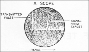
Scope. Radars came with
different kinds of display scopes.
U.S. Navy. Via Ibiblio.org
The A
scope was a simple oscilloscope displaying the strength of the
return signal as a function of distance.
U.S. Navy. Via Ibiblio.org
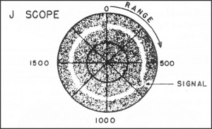
The J
scope was a modification of the A scope that displayed in polar
coordinates, with distance as angle and strength of return as
radius. This allowed a longer sweep and provided superior distance
resolution.
The B
scope plotted direction as the horizontal coordinate and distance
as the vertical coordinate, with significant returns shown as
"pips" or bright spots on the scope. It was the first scope
to provide a two-dimensional map of the search area, albeit a
distorted map that required some experience to interpret
correctly. It used persistent phosphors to take maximum advantage
of the display format.
 H scope. U.S. Navy via ibiblio.org |
 O scope. U.S. Navy via ibiblio.org |
A later development of the B scope was the H scope, which gave a double return where the vertical separation of the two pips was an indication of altitude. The similar O scope was used in air intercept radars and gave an altitude indication for the aircraft carrying the radar.
The C
scope resembled the B scope but plotted direction horizontally and
altitude vertically. It was always used in conjunction with other
types of scopes that gave range information.
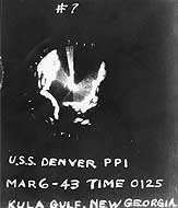
The PPI
or Plan Position Indicator scope combined features of the J scope
and B scope. It provided an undistorted two-dimensional map of the
area around the radar set, requiring little training for correct
interpretation. Altitude information was usually provided by a
separate C scope. The PPI is the radar scope that is familiar to
the public today.
U.S. Navy. Via Ibiblio.org
The G scope (Gunsight scope) was used in airborne
radars for night fighters and resembled a C scope, but the target
"blip" was smeared horizontally in proportion to distance. When
the "blip" was centered and its "wings" reached two vertical
markings on the scope, the fighter's guns were dead on target and
within range and the fighter could open fire.
Many early radars employed lobe switching, in which the antenna was split into two halves that were aimed in slightly different directions. The two return signals were plotted on an A scope but with the timing very slightly offset, producing a double-peaked return. When the antenna was aimed directly at the target, the two peaks were equal in height. This gave much better directionality than was possible with a single antenna.
Resolution: This is a measure of how well the radar can distinguish small targets located close together. About the only way to improve resolution was to use a narrower beam, since techniques such as lobe switching did little to improve resolution.
The very narrow beam required for high accuracy and resolution limits the sensitivity and scan rate. As a result, by the time war broke out in the Pacific, the Allies had already begun production of separate search and fire control radars, the latter having a narrow beam that scanned only in the direction of the target. The Japanese did not deploy their first specialized fire control radars until 1943.
Weight:
Radar weight was obviously important for airborne radars. It was
also important for seaborne radars because the radar tended to sit
high in the ship, which could reduce a small ship's overall
stability.
Production: Specifies
when the radar set became available and how many sets were
produced.
Both the Japanese and the Allies developed radar countermeasures
during the war, but Japanese radar countermeasures trailed behind
those of the Allies.
The Allies first recognized that the Japanese had significant
radar capability with the capture of the "Guadalcanal
radar" in August 1942. The Allies responded by dispatching
U.S. Navy XARD intercept receivers and U.S. Army SCR-587 search
receivers to the Pacific. The XARD was small enough to be carried
in a heavy bomber and could cover the spectrum between 50 to 1000
MHz (wavelengths of 30 to 600 cm). A flight by an XARD-equipped B-17 from Espiritu Santo to the Solomons in October
1942 failed to uncover any Japanese transmitters. Dedicated
"ferret" aircraft, B-24s
with a suite of radar detectors were soon sent to the Pacific, and
on 6 March 1943 these confirmed the presence of Japanese radar in
the Aleutians. Early
in the strategic
bombing campaign against Japan, one in four B-29s carried the
APR-4 intercept receiver, manned by an extra crewman dubbed the
"Raven", and a few aircraft carried ARR-5 communications search
receivers. These aircraft were the first to characterize the Taichi-6
early warning radar and several other fire-control radars. The
aircrew noted that the fire- and searchlight-control radars did
not seem particularly effective, and generally Japanese radar as
being three years behind their Allied counterparts.
The Japanese received schematics for the German Metox radar warning receiver, and manufactured more than 2000 sets. However, by the time these reached the fleet, the Allies had largely switched to microwave radar to which it was not sensitive.
Once radars were detected and characterized, they could be
attacked in one of three ways. Aircraft sometimes attacked the
radar sites, but they were difficult targets and were swiftly
repaired. Other countermeasures were jamming, to overwhelm
the receivers with noise, and spoofing, to produce
spurious signals that deceived the radar operators.
Both sides employed chaff, bundles of aluminum foil strips dropped from aircraft to produce false blips on the enemy's radar screens. The British called their version Window, while the Japanese knew it as deceiving paper (giman-shi). The Japanese version was invented by a Navy lieutenant commander, Sudo Hajime, and first used with some success to confuse Allied gunlaying radars in the Solomons in 1943. The Japanese successfully decoyed a few fighters away from the American carrier force at the Battle of the Philippine Sea, using chaff dropped from a lone Judy, but this had little effect on the outcome of the battle. The Japanese generally considered aluminum too scarce a resource for the production of large quantities of chaff, but it was used in small quantities throughout the remainder of the war and in larger quantities during the kamikaze raids at Okinawa. The Japanese generally dropped the chaff thirty miles from the target, and it was successful at blocking metric radar but not centimetric radar. It was also used with some success to confuse radar-controlled antiaircraft fire.
Both sides also experimented with electronic jamming of radar. The Allied efforts dated back to the Battle of Britain, received generous support, and became quite sophisticated as the war progressed. However, jamming was deliberately avoided early in the strategic bombing campaign, with the first extensive use being during the raid of 7 April 1945. Fully 247 APT-1 and APQ-2 jammers were carried by the raiding aircraft, along with "Rope" chaff (foil strips 400 feel long) against long-wavelength radar. The Japanese had not taken the precaution of spreading the operating frequencies of their fire-control radar, which were thus easily jammed. American raids thereafter carried increasing numbers of increasingly sophisticated jammers.The introduction of specialized "Guardian Angel" jammer aircraft coincided with a steep drop in losses to antiaircraft fire.
Naval air forces also made use of radar jamming, with the Enterprise air
group embarking Avengers
in early 1945 equipped with jamming equipment.
The Japanese experimented with jamming of radar during the Guadalcanal campaign, but
many of the scientists and technicians who could have improved
Japanese radar and radar countermeasures were drafted into the military.
Though not precisely a countermeasure, aircraft approaching a radar station from behind a mountain range were usually screened from detection until they crossed the range. This proved advantageous to the Japanese early in the New Guinea campaign, when radar was available only at Port Moresby. Japanese raids across the Owen Stanley mountains were often not detected until just minutes beforehand. The deployment of radar to Dobodura greatly improved early warning.
Once radar countermeasures came into use, the logical next step
was counter-countermeasures. The simplest was to spread the
operating frequencies of radars so that jammers had to cover more
of the spectrum. However, Allied aircraft in the Pacific were
little troubled by Japanese jamming, while the American postwar
report on air operations dismissed Japanese jamming as
nonexistent.
In addition to the alphabetical listings, we present
chronological tables that illustrate the development of radar by
each major power. This is intended as an aid to estimating what
radar capabilities were available at given times during the war.
The actual radar sets available for a given ship at a given action
can be difficult to pin down, since radar was a critical, highly
sensitive, rapidly evolving technology, and installation was often
dependent on a ship being refit at a time when sets were
available. Thus, during the Guadalcanal campaign, some but not all
of the Allied ships had SC and SG radar. The chronological
listings are an attempt to show when a particular set would have
begun to make its appearance in the Pacific, and on which ships or
in which settings.
Japanese radar were designated by Mark (Go), which indicated the intended use; Model (Kei/Kata/Gata); Modification (Kai); and Type (Shiki). Mark 1 was ground based search and early warning radar; Mark 2 was shipboard search and early warning radar; Mark 3 was shipboard fire control radar; Mark 4 was antiaircraft fire control radar; Mark 5 was panoramic indication/airborne/search radar; and Mark 6 was ground controlled interception radar. Type 1 was fixed radar, Type 2 was mobile radar, and Type 3 was portable radar. Type 4 may have referred to airborne radar. Mark and Type were combined into a single two-digit designation, such as 11 for fixed ground-based early warning radar. There is significant confusion in the English literature due to various translations of these terms, including the frequent translation of the designation as Type. We have used Type for the designation in spite of the potential for confusion, which exists in any case.
Japanese Army radar had designations based on acronyms for the
originating institution (Tama Research Institute) and the intended
use. Thus, Tachi indicated Tama ground-based radars, Tase
indicated Tama shipboard radars, and Taki indicated
airborne radars.
Tachi-1 searchlight direction radar
Tachi-2 searchlight direction radar
Tase-2
Type 4 antisubmarine radar
Type 11 early
warning radar
Type 12 early
warning radar
Type 13 air
search radar
Type 21
general purpose radar
Type 22
general purpose radar
Type
32
fire control radar
Type 42 fire
control radar
Type 6
Mark 4 Mod 3 airborne radar
| Set |
Type 21 |
Tachi-6 | Type 22 | Type 6 Mark 4 Mod 3 | Type 11 | Type 12 | Tachi-1 |
|---|---|---|---|---|---|---|---|
| Type |
General purpose |
Early warning | General purpose | Airborne | Early warning | Early warning | Searchlight |
| Range |
60 nm/100 km aircraft group 40 nm/70 km single aircraft 12 nm/20 km battleship |
125 mi/200 km aircraft group | 20 nm/35 km aircraft group 10 nm/17 km single aircraft 13 nm/24 km battleship |
75 nm/130 km ships | 75 mi/120 km single aircraft 155 mi/250 km aircraft group 10 mi/16 km ships |
30 mi/50 km single aircraft 60 mi/100 km aircraft group |
25 mi/40 km aircraft |
| Production |
40 | 350 | 300 | 2000 |
30 | 50 |
150 |
| 1942-4 |
BB Ise | ||||||
| 1942-6 |
Overseas | ||||||
| 1942-8 |
CV Shokaku |
New destroyers | Prototype | ||||
| 1942-10 |
Kongos | ||||||
| 1942-12 |
Prototype overseas | Prototype overseas | |||||
| 1943 |
Home islands and Formosa | ||||||
| 1943-1 |
Escort carriers |
||||||
| 1943-2 |
|||||||
| 1943-3 |
|||||||
| 1943-5 |
|||||||
| 1943-6 |
Light cruisers | ||||||
| 1943-7 |
Production | ||||||
| 1943-8 |
|||||||
| 1943-9 |
Ships Land |
||||||
| 1943-10 |
Yamatos | ||||||
| 1943-11 |
|||||||
| 1943-12 |
|||||||
| 1944-1 |
|||||||
| 1944-4 |
G4M "Betty" H8K "Emily" B5N "Kate |
Production | |||||
| 1944-8 |
|||||||
| 1944-9 |
Destroyers | ||||||
| 1945-6 |
| Set |
Tachi-3 | Tachi-2 | Tase-1 | Type 13 | Tachi-7 | Type 42 | Taki-1 Mod 2 |
|---|---|---|---|---|---|---|---|
| Type |
Antiaircraft fire control | Searchlight |
Early warning |
Air search | Early warning | Antiaircraft fire control | Airborne |
| Range |
25 mi/40 km aircraft | 20 mi/30 km aircraft | 110 mi/200 km aircraft group | 30-60 mi/50-100 km aircraft | 190 mi/300 km aircraft group | 2 mi/20 kmsingle aircraft 25 mi/40 km aircraft group |
8 mi/15 km submarine 30 mi/60 km large warships 55 mi/100 km fleet |
| Production |
150 | 25 | 30 | 1000 | 60 | 231 | 900 |
| 1942-4 |
|||||||
| 1942-6 |
|||||||
| 1942-8 |
|||||||
| 1942-10 |
|||||||
| 1942-12 |
|||||||
| 1943 |
Home islands and Formosa | ||||||
| 1943-1 |
Land | ||||||
| 1943-2 |
Army transports | ||||||
| 1943-3 |
Ships Submarines Land |
||||||
| 1943-5 |
Land | ||||||
| 1943-6 |
|||||||
| 1943-7 |
|||||||
| 1943-8 |
Land | ||||||
| 1943-9 |
Heavy bombers | ||||||
| 1943-10 |
|||||||
| 1943-11 |
|||||||
| 1943-12 |
|||||||
| 1944-1 |
|||||||
| 1944-4 |
|||||||
| 1944-8 |
|||||||
| 1944-9 |
|||||||
| 1945-6 |
| Set |
Tachi-4 | Tase-2 Type 4 | Tachi-18 | Taki-13 | Tachi-31 | Type 32 | Taki-1 Mod 4 |
|---|---|---|---|---|---|---|---|
| Type |
Antiaircraft fire control | Antisubmarine | Early warning | Altimeter | Antiaircraft fire control | Surface fire control | Airborne |
| Range |
12 mi/20 km aircraft | 1.2 mi/2 km periscope 6 mi/10 km surfaced submarine 20 mi/30 km surface warship |
125 mi/200 km aircraft group | 12 mi/20 km aircraft | 6 nm/12 km destroyer 20 nm/35 km battleship |
8 mi/15 km submarine 30 mi/60 km large warships 55 mi/100 km fleet |
|
| Production |
25 | 80 | 400 | 1500 | 49 | 60 | 300 |
| 1942-4 |
|||||||
| 1942-6 |
|||||||
| 1942-8 |
|||||||
| 1942-10 |
|||||||
| 1942-12 |
|||||||
| 1943 |
|||||||
| 1943-1 |
|||||||
| 1943-2 |
|||||||
| 1943-3 |
|||||||
| 1943-5 |
|||||||
| 1943-6 |
|||||||
| 1943-7 |
|||||||
| 1943-8 |
|||||||
| 1943-9 |
|||||||
| 1943-10 |
|||||||
| 1943-11 |
Land | ||||||
| 1943-12 |
Army transports | ||||||
| 1944-1 |
Home islands | Torpedo bombers | |||||
| 1944-4 |
|||||||
| 1944-8 |
Land | ||||||
| 1944-9 |
Coastal artillery | ||||||
| 1945-6 |
Heavy bombers |
The U.S. Army assigned SCR (Signal Corps Radio) designations to
its radars. The Navy assigned two-letter codes, sometimes with a
numerical model suffix, such as SC2. The Navy also sometimes
referred to its radars using a mark number, such as Mark 8. Radars
used by both services (including many airborne radars) usually had
a AN/APS number, though the AN (for Army-Navy) was often omitted.
| Set | CXAM | SC |
ASV Mark II | SCR-268 |
SCR-270 |
ASV Mark III (H2S) | FC |
|---|---|---|---|---|---|---|---|
| Type |
Early warning |
Search |
Airborne |
Antiaircraft fire control |
Early warning |
Airborne |
Surface fire control
|
| Range |
70 nm/130km bomber 50 nm/90km fighter 16 nm/30km battleship 12 nm/20km destroyer |
30 nm/60 km bomber 10 nm/20 km battleship 3 nm/6 km destroyer SC-1 doubled these ranges. |
20 mi/30 km destroyer 60 mi/100 km coastline Minimum range 1 mile (1.6 km) |
23 mi/37 km bomber | 140 miles/230 km | 100 miles/160 km coastline |
20,000 yards/18,000 meters shell splash 45,000 yards/41,000 meters bomber 12,000 yards/11,000 meters submarine
|
| Production |
20+ |
400 |
Thousands |
520 |
794 |
139 |
|
| 1941-12 |
Fleet carriers Six battleships Five cruisers |
Ships |
Sunderland Wellington Beaufort Hudson Liberator |
Corregidor |
Oahu Iba |
||
| 1942-3 |
|
||||||
| 1942-7 |
First sets in South Pacific |
||||||
| 1942-9 |
|||||||
| 1942-10 |
|||||||
| 1943 |
British heavy bombers |
||||||
| 1943-1 |
|||||||
| 1943-3 |
|||||||
| 1943-6 |
Cruisers |
||||||
| 1943-7 |
|||||||
| 1943-9 |
|||||||
| 1943-10 |
|||||||
| 1944 |
|||||||
| 1944-1 |
|||||||
| 1944-2 |
|||||||
| 1944-4 |
|||||||
| 1944-5 |
|||||||
| 1944-7 |
|||||||
| 1944-9 |
|||||||
| 1945 |
| Set | FD Mark 4 |
SD |
SA |
ASG |
SG |
Mark 8 |
SC-2 |
|---|---|---|---|---|---|---|---|
| Type |
Surface fire control | Early warning |
Air search |
Airborne |
Surface search |
Surface fire control |
Search |
| Range |
12,000 yards/11,000m shell splash 40,000 yards/37,000 meters bomber 12,000 yards/11,000 meters submarine 20,000 yards/18,000 meters destroyer 30,000 yards/27,000 meters battleship |
20 nm/37 km bomber | 40 nm/70 km bomber 30 nm/55 km fighter 12 nm/20 km battleship 8 nm/15 km destroyer |
18 mi/29 km submarine 40 mi/64 km cruiser 90 mi/140 km coastline Minimum range 400 yards/370 m |
15 nm/30 km low-altitude bomber 22 nm/41 km battleship 15 nm/30 km destroyer |
40,000 yards/36,600 meters battleship 31,000 yards/28,000 meters destroyer |
80 nm/150 km bomber 40 nm/70 km fighter 20 nm/40 km battleship |
| Production |
667 |
140 |
1490 |
5547 |
955 |
205 |
900 |
| 1941-12 |
|||||||
| 1942-3 |
|||||||
| 1942-7 |
First sets in South Pacific | Submarines |
|||||
| 1942-9 |
Destroyers Destroyer escorts Frigates |
||||||
| 1942-10 |
PBM
Mariner PBJ Mitchell PB4Y Liberator |
First sets in South Pacific |
|||||
| 1943 |
Battleships Cruisers |
Destroyers |
|||||
| 1943-1 |
|||||||
| 1943-3 |
Cruisers Destroyers |
||||||
| 1943-6 |
|||||||
| 1943-7 |
|||||||
| 1943-9 |
|||||||
| 1943-10 |
|||||||
| 1944 |
|||||||
| 1944-1 |
|||||||
| 1944-2 |
|||||||
| 1944-4 |
|||||||
| 1944-5 |
|||||||
| 1944-7 |
|||||||
| 1944-9 |
|||||||
| 1945 |
| Set | SK |
SF |
SJ |
SM |
ASD |
SCR-584 |
ASH |
|---|---|---|---|---|---|---|---|
| Type |
Air search |
Surface search |
Surface search |
Fighter direction |
Airborne |
Antiaircraft fire control |
Airborne |
| Range |
100 nm/190 km bomber 75 nm/140 km fighter 30 nm/55 km battleship 13 nm/24 km destroyer |
12 nm/22 km battleship 8 nm/15 km destroyer |
12 nm/22 km battleship 8 nm/15 km destroyer |
50 nm/90 km bomber 25 nm/50 km battleship |
25 mi/40 km 5000 ton ship | Detection at 50 nm/90 km Automatic tracking at 15 nm/30 km |
5 nm/9km aircraft 15 nm/30 km submarine 30 nm/55 km merchant ship 75 nm/140 km coastline |
| Production |
325 |
1655 |
300 |
49 |
5720 |
1700 |
|
| 1941-12 |
|||||||
| 1942-3 |
|||||||
| 1942-7 |
|||||||
| 1942-9 |
|||||||
| 1942-10 |
|||||||
| 1943 |
|||||||
| 1943-1 |
Ships |
||||||
| 1943-3 |
Frigates Corvettes |
Submarines |
Prototype on CV Lexington |
||||
| 1943-6 |
PV-1 Ventura | ||||||
| 1943-7 |
Europe |
||||||
| 1943-9 |
Fleet carriers |
||||||
| 1943-10 |
TBF Avenger | ||||||
| 1944 |
|||||||
| 1944-1 |
|||||||
| 1944-2 |
|||||||
| 1944-4 |
|||||||
| 1944-5 |
|||||||
| 1944-7 |
|||||||
| 1944-9 |
|||||||
| 1945 |
Philippines |
| Set | SL |
FD Mark 12 |
SCR-602 |
SU |
APS-15 | SO |
APS-6 |
|---|---|---|---|---|---|---|---|
| Type |
Surface search |
Fire control |
Early warning |
Surface search |
Airborne |
Surface search |
Airborne gunsight |
| Range |
15 nm/30 km low-flying bomber 20 nm/35 km cruiser 13 nm/24 km destroyer 10 nm/20 km submarine |
45,000 yards/41,000 meters bomber 40,000 yards/37,000 meters battleship |
70 miles/110 km bomber | 20 nm/40 km battleship 15 nm/30 km submarine |
15 nm/28 km harbor buoys 40 nm/74 km 5000-ton ship 95 nm/176 km large coastal city Minimum range 200 yards/180 m |
15 nm/28 km low-flying bomber 20 nm/37 km warships 5 nm/9 km submarines |
8,000 yards/7300 m fighter 10,000 yards/9100 m bomber 15 mi/25km submarine 30 mi/50 km merchant ship 65 mi/105 km coastline Minimum range 120 yards/110 m |
| Production |
1309 | 650 |
522 |
6089 |
791 | ||
| 1941-12 |
|||||||
| 1942-3 |
|||||||
| 1942-7 |
|||||||
| 1942-9 |
|||||||
| 1942-10 |
|||||||
| 1943 |
|||||||
| 1943-1 |
|||||||
| 1943-3 |
|||||||
| 1943-6 |
|||||||
| 1943-7 |
|||||||
| 1943-9 |
|||||||
| 1943-10 |
Destroyer escorts |
||||||
| 1944 |
Mark 37 directors (5"/38 guns) |
||||||
| 1944-1 |
Pacific |
Destroyer escorts |
|||||
| 1944-2 |
Heavy bombers |
PT boats LCC |
|||||
| 1944-4 |
Single-seat night fighters |
||||||
| 1944-5 |
|||||||
| 1944-7 |
|||||||
| 1944-9 |
|||||||
| 1945 |
Mobile land |
| Set | SCXR-720 |
ST |
SP |
Mark 27 |
SV |
AN/APQ-7 |
|---|---|---|---|---|---|---|
| Type |
Airborne gunsight |
Torpedo fire control |
Fighter direction |
Surface fire control |
Air search |
Radar bombsight |
| Range |
10 mi/16 km bombers at 10,000' (3000 m) 5 mi/8 km fighters at 17,000'/5200 m Minimum 250'/75mm |
8 nm/15 km battleship 3 nm/6 km submarine |
35 nm/65 km low-flying bomber 70 nm/130 km bomber at altitude 40 nm/70 km fighter 35 nm/65 km battleship 25 nm/45 km destroyer 15 nm/30 km submarine |
40,000 yards/36,600 m cruisers 10,000 yards/9100 m submarines Minimum range 200 yards/180 m |
7.5 mi/12 km bombers at 30,000 '/9100 m 10 mi/16 km bombers at 10,000 '/3000 m 12 mi/19 km fighters at 10,000 '/3000 m 12.5 mi/20 km battleship 15 mi/24 km cruisers 10 mi/16 km destroyers 7.5 mi/12 km surfaced submarine Minimum range 400 yards/360 meters |
30 miles/50 km |
| Production |
254 |
300 |
||||
| 1941-12 |
||||||
| 1942-3 |
||||||
| 1942-7 |
||||||
| 1942-9 |
||||||
| 1942-10 |
||||||
| 1943 |
||||||
| 1943-1 |
||||||
| 1943-3 |
||||||
| 1943-6 |
||||||
| 1943-7 |
||||||
| 1943-9 |
||||||
| 1943-10 |
||||||
| 1944 |
||||||
| 1944-1 |
||||||
| 1944-2 |
||||||
| 1944-4 |
||||||
| 1944-5 |
P-61 Black Widow | |||||
| 1944-7 |
Submarines |
|||||
| 1944-9 |
Fleet carriers Battleships Cruisers Some destroyers |
|||||
| 1945 |
Essexes |
Battleships |
Submarines |
|||
| 1945-5 |
B-29B
Superfortress |
British radars were invariably given a three-letter type number, usually beginning with "2". (Types beginning with "1" were usually sonars.) There was no particular system to the numbering, and in particular, larger numbers were not necessarily later systems.
Note that certain U.S. systems were also provided to the British.
For example, FC was known in British service as the Type 284.
| Set | Type 271 | Type 279 |
Type 281 |
Type 286 |
Type 291 |
|---|---|---|---|---|---|
| Type |
Surface search |
Air search |
Early warning |
Search |
Search |
| Range |
11 nm/20 km battleship 10 nm/19 km heavy cruiser 8 nm/15 km destroyer 6 nm/11 km frigate 3.5 nm/6.5 km PT boat 3 nm/6 km submarine |
65 to 95 nm/120 to 175 km at 16,000'/5000 m 27 to 40 nm/50 to 75 km at 3000'/370 m 16 to 24 nm/30 to 44 km at 1000'/300 m 5 to 8 nm/9 to 15 km at 100'/30 m |
100 nm/160 km at 16,000 '/5000 m 44 nm/90 km at 3000 '/370 m 25 nm/45 km at 1000 '/300 m 8 nm/15 km at 100 '/30 m |
8 nm/15 km cruiser 4-7 nm/7-13 km destroyer 1-1.5 nm/2-3 km submarine 2 nm/4 km PT boat 15 nm/30 km aircraft at 1000'/300 m 25 nm/45 km aircraft at 16,000'/5000 m |
35 nm/65 km aircraft at 10,000 '/3000 meters 30 nm/55 km aircraft at 5000 '/1500 meters 15 nm/30 km aircraft at 1000 '/300 meters 9 nm/17 km battleship 6 nm/11 km destroyer 3 nm/5 km submarine |
| Production |
350 |
||||
| 1941-12 |
Frigates Corvettes Destroyers (Type 272) Cruisers (Type 273) Battleships (Type 273) |
Ships |
Cruisers Battleships |
Destroyers |
Destroyers Escorts Submarines |
| 1943 |
Type 271Q |
||||
| 1943-4 |
|||||
| 1944 |
|||||
| 1944-9 |
Type 272P |
||||
| 1945 |
| Set | Type 277 | Type 276 |
Type 293 |
|---|---|---|---|
| Type |
Search | Search |
Fire control |
| Range |
23 nm/40 km battleship 20 nm/37 km heavy cruiser 18 nm/33 km destroyer 15 nm/28 km frigate 10 nm/18 km submarine 30 nm/55 km aircraft |
16 nm/30 km battleship 14 bn/26 km heavy cruiser 12 nm/22 km destroyer 10 nm/19 km frigate 7 nm/13 km PT boat 5 nm/9 km submarine 14 nm/20 km aircraft |
15 nm/30 km aircraft at 10,000 '/3000 m 12 nm/20 km aircraft at 5000 '/1500 m 10 nm/18 km aircraft at 1000 '/300 m 17 nm/31 km battleship 12 nm/22 km destroyer 4 nm/7 km submarine |
| Production |
|||
| 1941-12 |
|||
| 1943 |
|||
| 1943-4 |
Ships | ||
| 1944 |
Destroyers |
||
| 1944-9 |
|||
| 1945 |
Destroyers |
References
FTP-217 (1943-8-1; accessed 2012-6-14)
Library of Congress (2007; accessed 2011-6-1)
McFarland
(1998; accessed 2011-6-1)
Nakagawa
(1997)
Peattie (2001)
The Pacific War Online Encyclopedia © 2006-2014, 2016 by Kent G. Budge. Index
